


Edited by: Paz González Rodríguez
Madrid Health Service. Primary Care Paediatrics. Madrid . Spain
María Aparicio Rodrigo
Madrid Health Service. Primary Care Paediatrics. Complutense University of Madrid. Madrid . Spain
Last update: September 2025
More infoThe results of epidemiological studies should be expressed in terms of measures of health or disease. This article reviews the key frequency, risk and impact measures, which can be estimated using proportions, ratios or rates, depending on the specific context. It discusses which measures are appropriate for a study based on its design. Cross-sectional studies serve to estimate the prevalence; cohort studies allow calculation of the incidence, relative risk and attributable fractions; case-control studies use the odds ratio and clinical trials determine the relative risk, absolute and relative risk reductions and number needed to treat (NNT). The article also outlines criteria for the interpretation of these measures, supported by specific examples.
Los resultados de los estudios epidemiológicos deben ser expresados en forma de medidas de salud o enfermedad. En este artículo repasamos las principales medidas de frecuencia, riesgo e impacto, que se pueden estimar usando, según el caso, proporciones, cocientes o tasas. Veremos que, a cada estudio, en función de su diseño, le corresponden diferentes medidas. En un estudio transversal estimaremos la prevalencia; en un estudio de cohortes la incidencia, el riesgo relativo y las fracciones atribuibles; en un estudio de casos y controles la odds ratio; en un ensayo clínico el riesgo relativo, las reducciones absoluta y relativa del riesgo y el número necesario a tratar. Presentaremos los criterios de interpretación de todas estas medidas con ejemplos concretos.
The results of epidemiological studies must be presented in terms of health or disease measures, expressing frequencies, differences, association, risk or impact. How results are presented depends on the study design and, above all, the characteristics of the variable or variables of interest. Based on the type or types of variables at hand, we can use different epidemiological measures.
In epidemiology, the simplest scenario is the study of two discrete dichotomous variables. This scenario corresponds to the usual hypothesis concerning the association between the presence/absence of a specific exposure factor and the presence/absence of disease. To analyze this association, we have a series of frequency, risk and impact measures at our disposal.
Frequency measures describe the distribution of the disease in the population and they are useful to describe the disease as a first step in the research process. Measures of association are useful for understanding the relationship of the disease with risk factors, its magnitude and its importance. Impact measures are useful for estimating the potential repercussions of preventive or therapeutic interventions.
Another common scenario is the assessment of the association between one discrete variable and one continuous variable. This scenario corresponds to studies that assess the impact of an exposure factor (for instance, treatment versus placebo) on a quantifiable effect measured over a continuous range of values (for instance: blood pressure); in this type of study, results will be expressed in terms of the differences between groups in measures of central tendency (mean, median) and measures of dispersion for the continuous variable.
Preliminary conceptsWe will start by reviewing some arithmetic concepts on which epidemiological measures are based: proportion, ratio and rate.1
A proportion is a number of observations with a given characteristic (e.g., neonates with congenital malformations) divided by the total number of observations, with and without that characteristic, in a specific group (for instance, all neonates born in a given period with or without malformations). In proportions, the numerator is a subset of the denominator. The result is expressed as a decimal value ranging between 0 and 1 (0 to 100 when expressed as a percentage) and is equivalent to the probability of the evaluated characteristic.
A ratio or quotient is the result of the division of any two numbers in which the numerator is not a subset of the denominator. One example is the body mass index, which is the quotient of the weight in kilograms and the height in square meters.
A rate is generally defined as the change in magnitude of one variable per unit change in the other variable. Thus, it is a dynamic measure that allows us to measure not only the probability of the characteristic we are evaluating, but also the speed with which it occurs. For instance, the number of disease relapses as a function of the duration of follow-up is expressed as a rate.
The term odds does not have a suitable direct translation to Spanish (“razón de posibilidades”, “razón de ventajas”), so it is used untranslated. It refers to the quotient obtained by dividing the probability of an event (P) by the probability of the event not happening (1−P).
Frequency measuresIncidence and prevalence are the most widely used measures of morbidity in the medical literature.1,2 It is important to differentiate them.
The prevalence is the number of individuals that have a given disease or characteristic at a specific point in time divided by the population at risk at that time. If we measure the individuals that have the disease or characteristic at any point during a specified time period, we obtain the period prevalence. The prevalence is usually measured through cross-sectional studies and expressed as a proportion. For instance, if there are 250 children with obesity among a total of 1000 managed at a primary care center, the prevalence of obesity is 0.25 (25%).
The incidence is the number of new cases that have occurred over a time interval divided by the number of the population at risk at the start of the interval. This information is usually obtained through cohort studies and expressed as a proportion or rate. We can differentiate between two types of incidence: cumulative incidence (proportion) and incidence density (rate).
The cumulative incidence is a proportion calculated by dividing the number of new cases by the size of the population at risk. It is used when the disease is not expected to occur more than once in any given subject and the population at risk remains fixed. For example, if 20 cases of meningitis are diagnosed in a year in a population of 100 000 children aged less than 5 years, the cumulative incidence is 0.0002 (or 2 per 10 000).
The incidence density is a rate calculated by dividing the number of new cases by the sum of the time each subject was followed up totaled for the entire population at risk (e.g., months or years). It is used when the risk of disease is proportional to the duratioeffn of follow-up, each subject can correspond to more than one case and the duration of follow-up may vary between subjects. For example, if we measure the frequency of gastroenteritis in children attending a child care center in relation to the time they have been enrolled in the facility and we record 10 new episodes of gastroenteritis in a set of 25 children (2 children had more than one episode) who had been enrolled in the center for a mean of 2 mo (50 mo in total), the incidence density of gastroenteritis would be of 0.2 cases (10/50) per child and month of exposure.
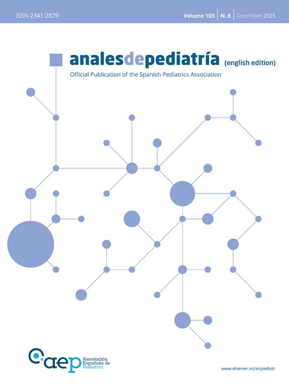
The prevalence and the incidence offer complementary information (Fig. 1). A disease with a high incidence but also either a high mortality rate or a high cure rate will have a low prevalence in the population. On the other hand, a disease with a low incidence that also has either a low mortality or a low cure rate (tends to become chronic) may have a high prevalence. The effect of mortality on the prevalence can affect the characteristics of the samples selected to conduct a study, as the population of subjects eligible for inclusion in a study of prevalent cases would result in the selection of patients with a better prognosis and a lower frequency of risk factors compared to the population of subjects eligible for a study of incident cases.
Risk measures (association)
In epidemiology, the concept of risk refers to the probability that individuals exposed to certain factors develop an outcome of interest to a greater or lesser extent. Tables 1 and 2 present the formulas for the calculation of the main risk measures: the relative risk (RR) and the odds ratio (OR).


The RR is calculated by dividing the incidence in the group of subjects exposed to a given risk or protective factor by the incidence in the unexposed group.3 It can only be calculated in longitudinal studies and is a measure of the strength of the association between exposure and disease. It can take values ranging from 0 to infinite, with values of less than 1 for protective factors (the incidence is smaller among the exposed) and greater than 1 for risk factors (the incidence is higher among the exposed); a RR of 1 is the null value (identical risk in both groups), and a greater distance of the RR from 1, either above or below, reflects a stronger association.
In studies in which the duration of follow-up varies between subjects, rather than using the cumulative incidence, risk is calculated based on the incidence density, in which each subject is reflected in the denominator based on the amount of time they followed up. In such instances, risk is estimated using the incidence density ratio (IDR), which is the quotient of the incidence densities of the exposed and unexposed groups.
In studies that do not have a longitudinal design (case-control studies), since the incidence cannot be calculated, it is not possible to calculate the relative risk.4 In such cases, the risk is estimated by means of the OR, which compares the odds of exposure (the probability of exposure to a risk factor divided by the probability of not being exposed) in the case group (with the disease) and the odds of exposure in the control group (without the disease) by dividing one by the other. The interpretation of the OR is similar to the interpretation of the RR: 1 is the null value, values of less than 1 indicate decreasing risk and values greater than 1 increasing risk. It should be taken into account that the RR and OR only yield similar values if the frequency of the disease or condition under study is very low.
Another measure of risk used in survival studies is the hazard ratio.5 This measure is calculated in survival studies (in which the response variable is the time elapsed until the event occurs) and is the quotient of the conditional risks in the groups compared throughout the follow-up. The interpretation of the hazard ratio is similar to that of the RR or the OR, with a value of 1 indicating absence of risk or association, greater values increased risk and lesser values decreased risk.
Impact measuresAlthough the measures discussed above allow us to estimate the risk generated by an exposure facture of a given effect or disease, they do not provide information regarding the impact that the exposure may have on the set of existing cases in a population. This information is obtained through other measures, such as the risk difference or the attributable proportion (Table 1).3,6,7
Both measures estimate the absolute impact of exposure on the incidence of an event in the exposed group or the total population. They are used to assess the clinical or public health importance of an exposure factor and inform us of the percentage by which the incidence would decrease if said factor were to be removed. Thus, there are very useful in both clinical practice and public health for quantifying the potential impact of different interventions.
The risk difference (RD) is calculated by subtracting the incidence in the unexposed group from the incidence in the exposed group. The RD is a measure of absolute impact that takes values ranging from 0 to 1 (or 0 to 100 if expressed as a percentage), where 0 is the null value representing the absence of differences. The RD offers information that is independent from the relative risk and may vary between different groups of patients based on the specific risk of each group. Thus, we may find that factors with a very high relative risk yield very low risk differences because the risk in the population (outside of the contribution of the factor at hand) is very low. For example: the incidence of admission due to bronchiolitis in a group of infants who attended daycare was 0.02 or 2%, compared to only 1% in infants cared for at home; the relative risk indicates that the increase in risk is 50% (RR, 0.5), while the risk difference is as small as 1% (RD, 0.01).
The attributable fraction among the exposed (AFe), also known as attributable risk, etiologic fraction or attributable proportion is defined as the proportion of new cases of disease in the group of exposed subjects that can be attributed to the risk factor of interest. It is calculated by dividing the previously calculated risk difference by the incidence in the exposed group. An extension of this measure is the population attributable fraction (PAF), which applies the proportion of new cases to the entire population, that is, to both the exposed and unexposed subjects. When the factor under consideration is a preventive factor, the estimated impact measure is known as the preventable fraction, which corresponds to the proportion of cases among the exposed that could be prevented by applying the preventive factor. These impact measures cannot be estimated directly from data obtained through a case-control study, as this design does not yield incidence estimates. However, we can use the OR as a substitute of the RR to estimate impact, as long as the prevalence of the disease is low (in which case, OR values are close to RR values; for more frequent diseases, formulas are available to estimate the RR based on the OR).
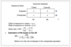
The results of clinical trials tend to reflect the beneficial effect of therapeutic interventions that reduce risk in the exposed group (Table 3). Thus, in this context, the risk difference, referred to by the alternative term of absolute risk reduction (ARR), is calculated in the opposite order, subtracting the risk in the intervention group from the risk in the control group. Dividing the ARR by the risk in the control group yields the relative risk reduction (RRR), which expresses the proportion by which the risk decreased in the intervention group relative to the control group. Another impact measure that is applicable to this type of studies and is of great clinical interest is the number needed to treat (NNT),8 which is the inverse of the ARR (1/ARR) and represents the number of patients that need to be treated with the given intervention for one patient to benefit, preventing one instance of an unfavorable outcome.
Analysis of clinical trials.
| Response rate in intervention group | Pi=no events intervention grouptotal subjects intervention group |
| Response rate in control group | Pc=no events control grouptotal subjects control group |
| Relative risk reduction | RRR=Pc-PiPc |
| Absolute risk reduction | ARR = Pc −Pi |
| Number needed to treat | NNT=1ARR |
There are other impact measures applicable to observational studies, which are not discussed here, that interested readers can be informed about by consulting other sources.9,10
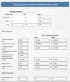
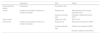
Selection of epidemiological measures based on study designTable 4 presents the measures of frequency, risk and impact used most frequently based on the study design when the effect is measured by means of a dichotomous variable. Thus, in a cross-sectional study, we will estimate the prevalence, in a cohort study the incidence (cumulative incidence or incidence density), the relative risk (or incidence density ratio) and attributable fractions (among the exposed and population); in a case-control study, we cannot estimate frequency, but it is possible to estimate risk, with the OR lastly, in a clinical trial, we will calculate incidence measures, relative risk, absolute and relative risk reductions and the number needed to treat.
Frequency, risk and impact measures for nominal dichotomous variables.
| Frequency | Risk | Impact | |
|---|---|---|---|
| Cross-sectional design | Prevalence | Prevalence ratio | |
| Cohort | Incidence (cumulative incidence or incidence density) | Relative risk | Attributable fraction among exposed (AFe) |
| Incidence density ratio | Population attributed fraction (PAF) | ||
| Case-control | Odds ratio (OR) | AFea, PAFa | |
| Clinical trial | Incidence (cumulative incidence or incidence density) | Relative risk | Absolute risk reduction (ARR) |
| Incidence density ratio | Relative risk reduction (RRR) | ||
| Number needed to treat (NNT) |
When the outcome measure of a study is a quantitative variable, estimating the mean difference or difference in means between the study groups is, in itself, a measure of association or impact (e.g., the difference in the means of glycated hemoglobin in two groups of diabetic subjects managed with different insulin regimens).
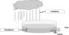
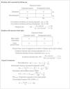
Figs. 2–4 show the calculation of measures performed with an online calculator, Calcupedev,11 for data obtained through a cohort study, a case-control study and a clinical trial. The user only needs to enter the counts in the contingency table, and the software calculates the appropriate measures with the corresponding 95% confidence intervals (CIs). To explain CIs, we would first need to explain the basic concepts of inferential statistics, which falls outside the scope of this review.12 It is important to keep in mind that any study obtains information from a sample of subjects, which is only one of the countless possible samples of a population; so that any measure estimated with the obtained data yields but one estimate among all the possible estimates that could be made in the population. To determine the level of uncertainty, statistical methods are available to estimate the ranges of values near the obtained value which would include the real value in the population. Specifically, a 95% CI indicates that there is a 95% probability that the true value in the population is contained within its bounds. A more orthodox interpretation is that if one were to take an infinite number of samples from a population to estimate the parameter of interest and calculated the 95% CI for each, 95% of the CIs would contain the true population parameter.


With the data from the cohort study, shown in Fig. 2, we can interpret that the factor under study is a risk factor (RR > 1). We can state that we have a confidence greater than 95% that the factor under study is truly a risk factor because the CI (1.065–3.755) does not contain the null value for risk (“1”). In addition, we may interpret that 50% of the risk in subjects exposed to the risk factor (AFe, 0.50) and 25% of the risk in the entire population (PAF, 0.25) is attributable to the risk factor, although the estimate for the PAF is imprecise, because the 95% CI contains the null value for proportions (in this case, “0”).
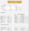
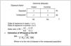
Based on the data for the case-control study presented in Fig. 3, we can interpret that the factor under study could be a risk factor (OR > 1); however, looking at the confidence interval, which includes the null value for risk (“1”), with the data obtained in this sample, we lack the confidence to declare it as such. Although the calculator estimates impact measures, the calculations were made under the assumption that the OR is equivalent to the RR, which may not be a valid assumption, since we do not know the incidence in the exposed and the unexposed populations (in this instance, we only know the risk of exposure in cases and unexposed controls).
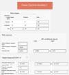
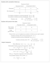
Based on the clinical trial data presented in Fig. 4, we can interpret that the therapeutic intervention reduces the risk of the outcome of interest, with an absolute risk reduction of 20%. We see that the CI does not contain the null value for the difference of proportions or means (“0”). Therefore, we have a level of confidence greater than 95% that the treatment is efficacious. In addition, we can see that in relative terms, the risk decreases by 50% compared to the control group (relative risk reduction). Lastly, the software calculates the number needed to treat, which can be interpreted as needing to treat five patients with the therapeutic intervention for one patient to improve in comparison to the control group; the CI informs us, with a level of confidence of 95%, that one in four treated patients would benefit in the best-case scenario, compared to one in 14 patients in the worst-case scenario.
FundingThis research did not receive any external funding.
The authors have no conflicts of interest to declare.
María Salomé Albi Rodríguez, Pilar Aizpurua Galdeano, María Aparicio Rodrigo, Nieves Balado Insunza, Albert Balaguer Santamaría, Carolina Blanco Rodríguez, Jaime Javier Cuervo Valdés, María Jesús Esparza Olcina, Sergio Flores Villar, Garazi Fraile Astorga, Javier González de Dios, Paz González Rodríguez, Rafael Martín Masot, María Victoria Martínez Rubio, Begoña Pérez-Moneo Agapito, María José Rivero Martín, Álvaro Gimeno Díaz de Atauri, Laura Cabrera Morente, Elena Pérez González, Juan Ruiz-Canela Cáceres.